 |
 |
11B Spectrum Processing
NMR Tubes for Boron NMRIf you need a cleaner and better-looking 11B spectrum, please order a 5 mm quartz NMR tube from Wilmad, either 507-PP-7QTZ or 528-PP-7QTZ. These tubes don't give a broad background B11 signal from the normal Pyrex tube. Further information on removing or reducing background signal in 11B and 29Si NMR can be found here.
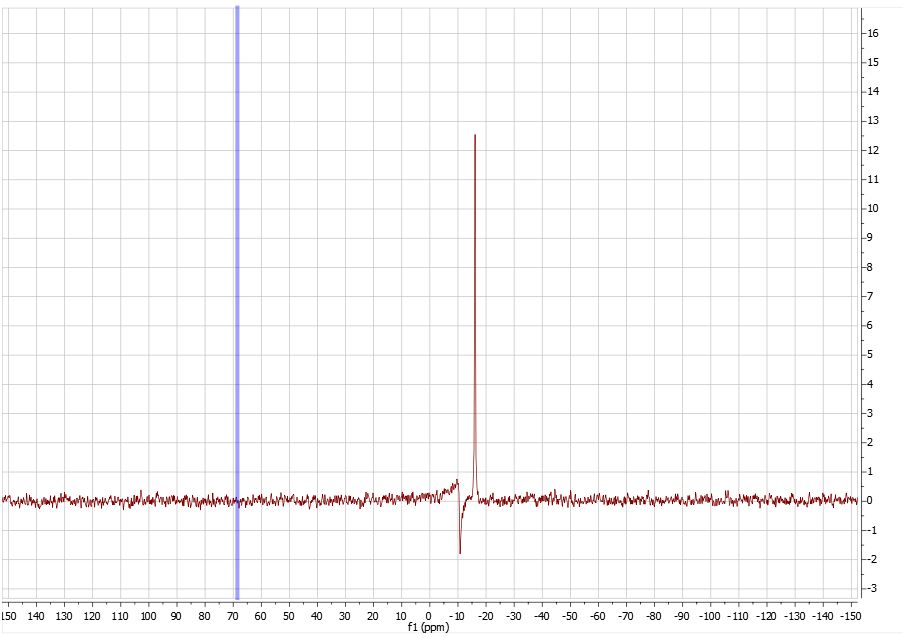
In general, the spectral window when collecting data should not be too wide, but in this case where the background signal is broad and significant, the width should enclose the entire broad profile and leave ~10-20% of baseline at each side. Otherwise, the tail of the broad profile will fold back into the spectral window from the other side and complicate baseline correction.
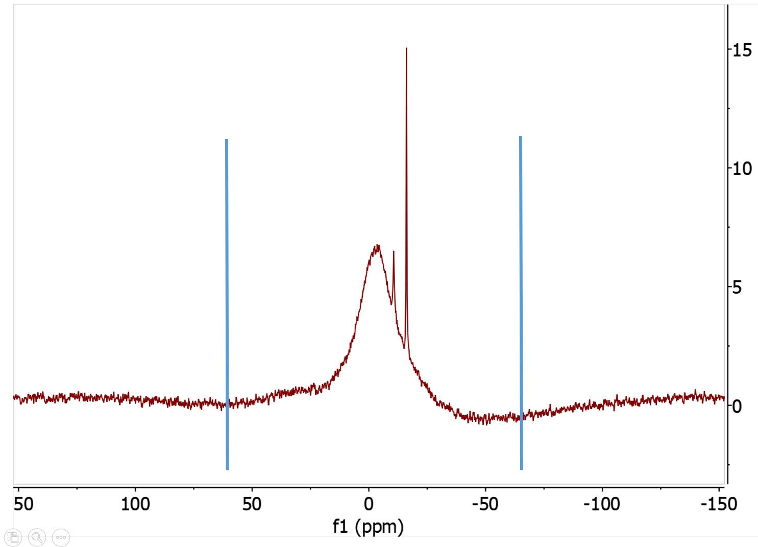
The two blue lines indicate a proper window size (under Acquisition) to enclose the entire broad signal. You can set the width by ppm values in Acquisition panel, or with the two cursor lines shown to enclose the region, enter movesw in the command line, then recollect the data.
We'll update other experimental methods that help mitigate this problem to some extent. One approach is to use a spin echo (90-180-Acq) with a delay in-between the pulses to wait for the broad signal to die out before data collection. But, the proper NMR tube above remains the top option for removing most of the broad background.
The following are the steps to remove the broad background signal during processing. This trick only works well if relatively sharp and strong 11B signals from the sample sit on top of the broad background signals coming from a normal NMR tube and possibly the glass insert of the probe. The processing steps include left-shifting (discarding initial points) the FID before processing and applying either linear prediction (LP) of the initial points before FT or a large first-order linear phase correction to remove phase distortion and rolling.
Steps to Remove/Reduce the Broad Background Signal with Processing
1. Process data and apply window function. In Mnova, open the fid file and process it. Go to Processing → Apodization and adjust the exponential window function and use a broadening amount that smooths the peaks but doesn't broaden them too much.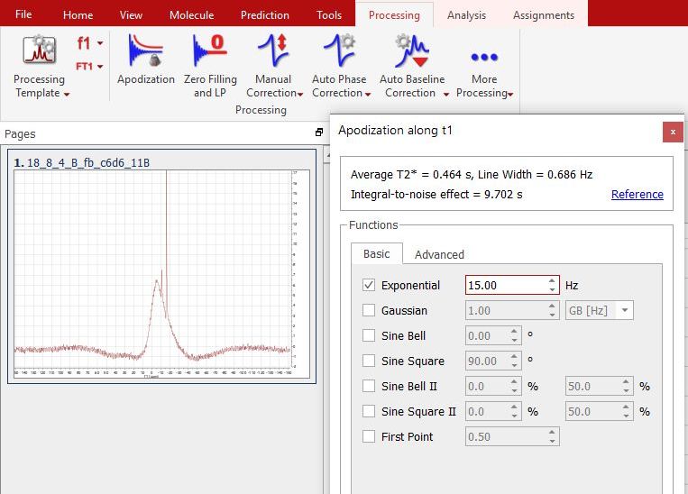
2. Phase the spectrum. Go to Processing → Manual Phase Correction and phase the spectrum. Autophase may not work well here.
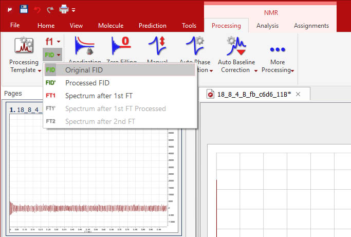
3. Go to Processing → FID to display original time-domain FID data. Click near the bottom axis of the spectrum display window and change the unit to point. Switch between second and point and check how many points correspond to ~0.15 msec or less (likely within the first ~20 points). You need to zoom in the initial FID. This gives you an idea how many points to left shift and discard below.
4. Left-shift FID. Go to Processing → More Processing → FID Shift ... Apply a left shift of -10 to -20 points (negative). With our default experiment setup, -20 points is a good start. But, ultimately it is the initial time we are dealing with and the points vary according to spectral width and acquisition time. The goal is to remove the first ~0.15 msec of the FID which corresponds to the broad background signal. It is assumed the signals of your interest last much longer and are fairly sharp.
5. Once the FID is left-shifted, go to Processing → FT1 (upper left corner) to show the FT spectrum if it isn't displayed. The spectrum should change with the broad signal greatly reduced. However, the peak phase needs to be adjusted.
6. Adjust PH0. Go to Processing → Manual Phase Correction. Watch a strong peak and adjust PH0.
7. Use linear prediction to fill in initial points. Use linear prediction (LP) to fill in the initial data points that are discarded. To do this, after the FID left shift, go to Processing → Zero Filling and LP and check "Backward", fill in From and To. If 20 poinst are left shifted, fill in -20 for From and 0 for To. The FT spectrum should show in-phase signals. Adjust PH0 if needed.
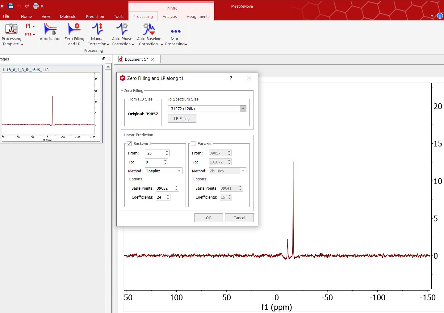
Backward linear prediction to fill in initial points followed by FT. Note 1st order correction isn't needed or is small.
8. Baseline correction: All baseline correction should be done after proper phasing. Select Manual Correction under Processing → Auto Baseline Correction. In manual mode, select one among the few choices there. The goal is to remove the baseline rolling and offset without taking out the signals of interest. A blue line indicates the baseline curve to be taken out from the spectrum. Watch this line closely as you make the function choice or adjust parameters. Try all the choices and see which one is the best.
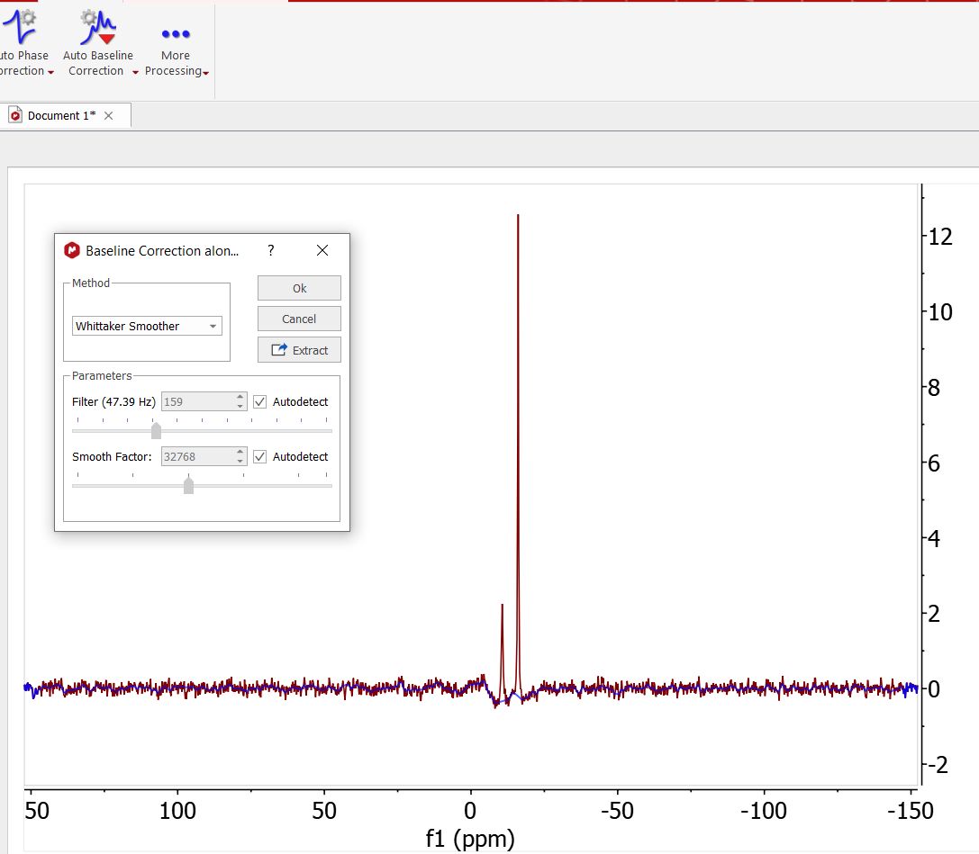
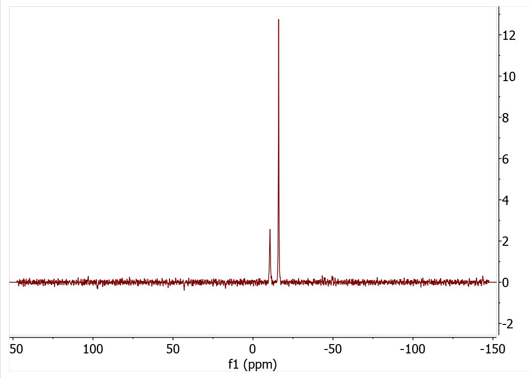
Final spectrum after Whittaker Smoother baseline correction. Other functions may work better in other cases depending on the baseline distortion.
Note: Alternatively, you may adjust PH1, first-order phase instead of LP, after left shifting the FID. In this example, the results of the two approaches are very similar. First, put pivot line on the strong peak where you made PH0 adjustment above. The theoretical correct PH1 amount should be points-shifted * 360-degree. That is, if the FID is left shifted by -20 points, PH1 should be 20*360 = 7200. Enter this value in PH1 field, but likely there will be baseline rolling due to other unrelated broad profiles. This can be dealt with baseline correction later. If not, a much smaller PH1 should be tried.
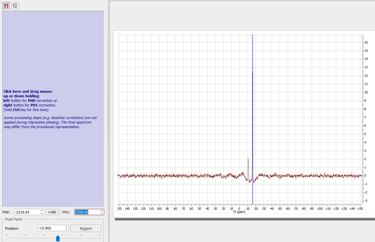
Spectrum after 7200 degree PH1 correction
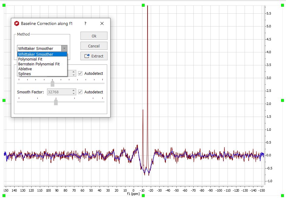
Baseline correction
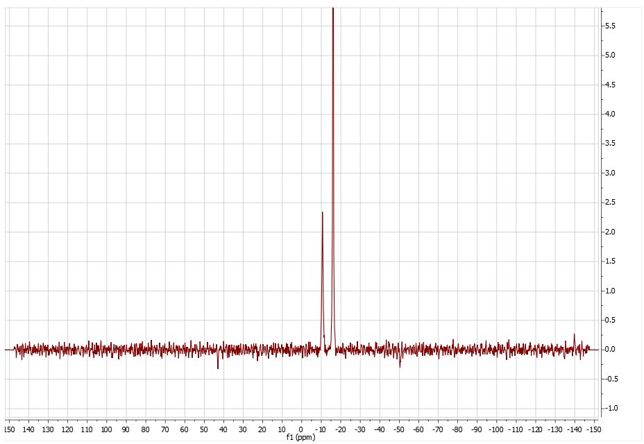
Final spectrum
Updated, 2019, H. Zhou