 |
Diffusion NMR Data Processing
Here we focus on the steps of DOSY processing with Mnova. Mestrelab has a general instruction for DOSY data
processing. In our practice, we have found more demands for diffusion constant measurements than visual display of molecular separation as shown
in a typical 2D plot of DOSY. The 2D DOSY contour plots, which are processed differently than curve fitting, tend to have much large room of uncertainty in the
diffusion constants shown along the Y axis. Here we give the steps using curve fitting for more consistent and accurate extraction of the diffusion constants.
By comparing the diffusion constants, we may also cluster peaks into groups that reflect different molecular sizes or shapes.
Step 1: Process DOSY array data.
Carefully apply proper window function, phasing, and baseline correction as usual.Note: You may use the first (most intense) spectrum to adjust the phase and baseline correction. The corrections should be applied to all spectra. However, a software bug has been observed that sometimes the phase correction isn't applied to one or two of the spectra in the array. Strangely, if the manual phase correction panel is engaged and the phase change is made there, suddenly the missing phase correction is applied to all spectra.
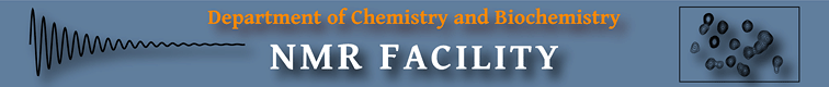
Step 2: Check parameters under array data table.
The values are automatically pulled from the parameter file (in procpar on Varian systems), but it's a good idea to make sure they are correctly entered. γ is the magnetogyric ratio of the spin beining detected (see a list here), Δ is the diffusion time (with corrections), δ is the gradient pulse duration, and k is the DAC to Gauss/cm (G/cm) conversion factor (DAC_to_G value).Step 3: Create integral graph.
Click Stacked, then Data Analysis, then New and select Integrals Graph. Then, manually define integrals around a peak or peaks. Press Esc key to exit an interactive mode. Click the manual integral picking icon to continue picking integrals for the current graph.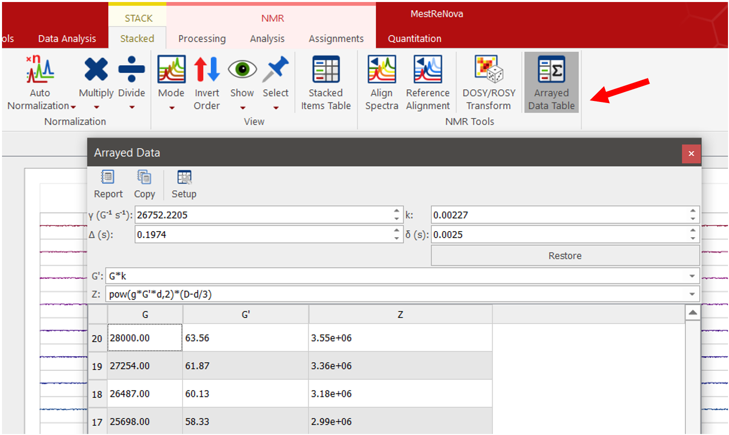 | 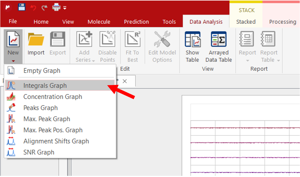 |
Step 4: Check fittings
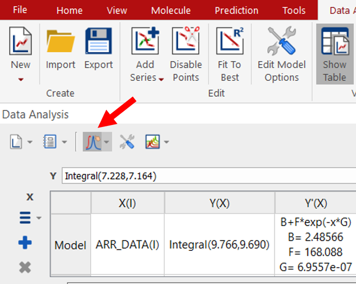
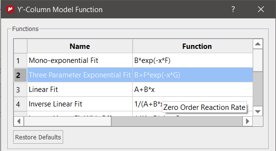
Integral curve fitting is automatically done with a three-parameter fit against a default model that appears to be y = B + F*exp(-x*G) where x is a product of known values and G is the diffusion constant. The best fit values are shown in the table above the graph for each integral list.The G values (should be renamed as D for diffusion constant) are remarkably consistent for a well-behaved homogeneous molecule even though the 2D DOSY contour plot may show obvious deviations. One main reason behind this difference is that integrals are used here, not peak heights or peak values point by point as used in the 2D DOSY analysis. Integrals capture more accurately the intensity attenuated by diffusion and are insensitive to peak shift during the experiment or peak overlapping.
Press Esc key to exist the interactive mode (to zoom in/out, for example). Click the manual integral picking button to continue to add new integrals. | 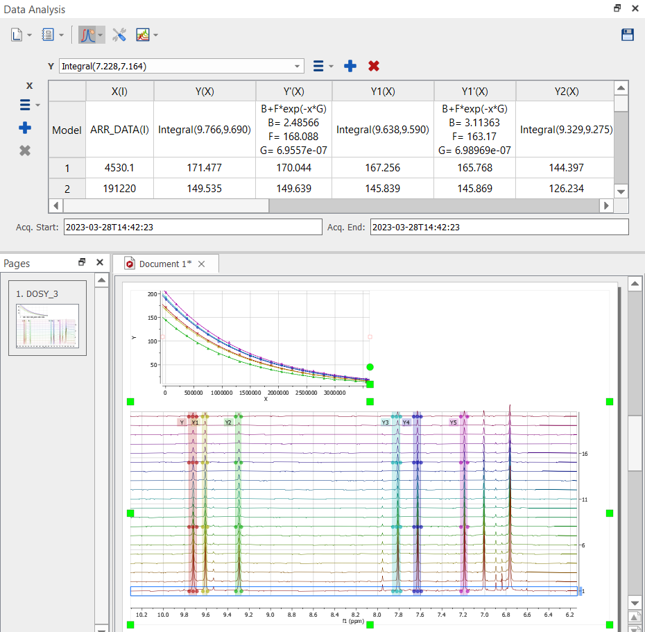
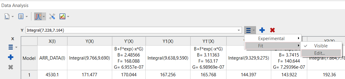
The G parameter in the general three-parameter fitting model is the diffusion constant and should be treated and renamed as D. The fitting curves do not start from and fall to the same values in the array. Therefore, in order to check similarity between the diffusion curves, the initial, largest values must be scaled to the same starting value. This is best done with an exported integral data table and curve fitting if desired. If the fitting data table, results and the integral picking icon and tools are not shown, click Data Analysis→Show Table. |
 |  |
Posted in March 2023 By H. Zhou