NMR Theory, UCSB Chem and Biochem NMR Facility

NMR Theory and Techniques

Note: During training and assisting students and researchers, I often find it helpful to go over some NMR theory which is usually picked up in bits and pieces sporadically over the years for most users. Evidently, this work has evolved into a much bigger project in a short time. I hope these materials will spur more interest in NMR and help all users, especially new ones, to broaden their skills and understanding of the NMR techniques. Some data shown here are synthesized, perfect data for illustration purposes. The data are generated with in-house written Tcl/Tk scripts, converted to nmrPipe binary data, and then processed with Mnova. Many common NMR terminologies are highlighted in bold. Since other aspects of the NMR techniques are covered in various lab classes, focus is given here to better understanding the mathematical and physical basis of various NMR observations and techniques. Some are very relevant to routine practice, especially in the design of NMR experiments and data interpretation. -- Hongjun Zhou, @UCSB, 01/2019

"I insist upon the view that 'all is waves'."
-- Erwin Schrödinger in Letter to John Lighton Synge (1959)

Transient NOESY: A Better Method of Measuring NOEs

Pulsed Field Gradients (PFG): Now You See It, Now You Don't

FID and FT

In an NMR experiment, what's actually detected and recorded by the instrument, specifically the receiver, is one (in 1D) or a series of (in an arrayed experiment, 2D, 3D ... ) free induction decay (FID) curves, as shown below. These data, however, are not smooth and continuous as shown here; they are recorded at fixed regular intervals a user can set. There are a known number of points in this graph. The display software connects these dots (detected data) to draw the smooth curve. The same goes for processed data or ANY experimental data of any kind whatsoever, except maybe by a stretch of imagination those recorded with superb analog devices. It's essentially always a limited number of data points. We call this limited "resolution" of the detection step. This is a trivial but important fact that affects many fields, not only NMR. We'll come back to this later regarding signal aliasing. However, data mostly can be interpolated, within a limitation, during processing in various ways without adding undesirable artifacts.

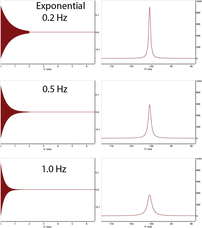
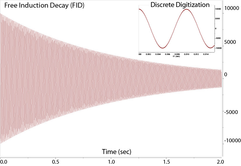FID of a single resonance at 100 Hz recorded for 2 secs

Data in frequency domain after FT

Shown above is an FID of a single resonance of a cosine wave with 100 Hz frequency recorded for 2 secs. The decay time constant (T₂ relaxation time) is 1 sec. The discrete recording interval is inverse to the spectral window in Hz (10000 Hz), at 0.0001 sec or every 0.1 msec. This leads to a raw data size of 2/0.0001=20000 pairs of complex data (20000 real + 20000 imaginary) points. The vertical axis is the intensity of the signal. Note the recorded signal ends abruptly due to the finite recording time relative to the long relaxation time (T₂) of the signal from the nuclear spin. The inset is the expanded, beginning portion of the actual discrete data points (real parts) digitized at regular intervals, every 0.1 msec.

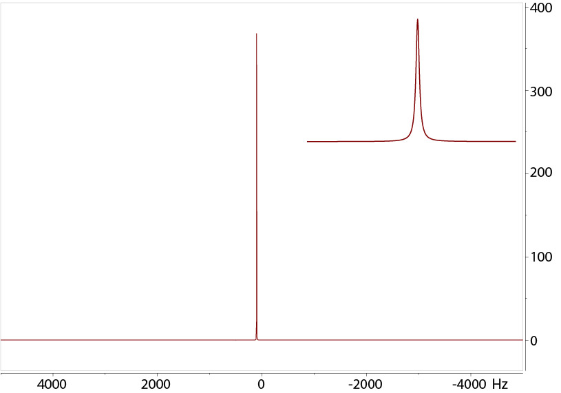
After data collection, the next step is to process the "time-domain" raw data above into the frequency domain through Fourier Transform (FT). This process involves multiple steps to give the best results. FT of the FID above gives the signal at 100 Hz. The inset is an expansion of the signal of a Lorentzian (or Cauchy) shape resulting from a simple exponential decay. The full linewidth at half height of the Lorentzian peak is Δν = 1/(πT₂) where T₂ is the relaxation time constant. The frequency domain spectrum is the one that is most used and reported. The unit of X-axis is often ppm, Hz, or point. For now, these units are not essential.

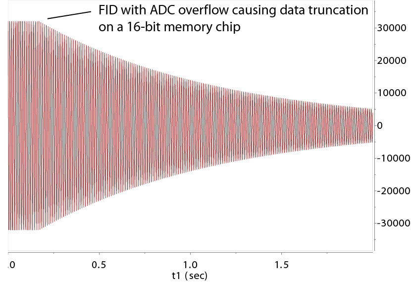
The receiver is a horizontally aligned coil that carries the induced current of the FID through the Faraday effect. The small current is amplified, then digitized into a 16-bit (or 32 bit) integer number and recorded. With Varian's standard 16 bit Analog-to-Digital Converter (ADC), the maximum "dynamic range" is -32,768 to +32,767. 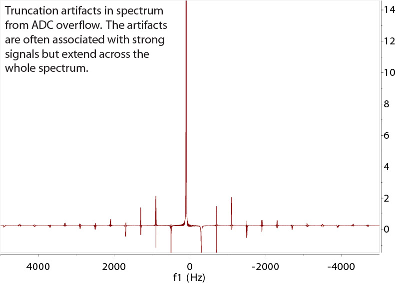An "ADC overflow" error message is given (on the Varian/Agilent system) if the maximum amplitude in the detection is outside this range. The receiver may be overflown from its own control before the analog-digital-converter (ADC) stage. ADC overflow means the signal is truncated at the very top which leads to "truncation artifacts" of a different kind from the case of sudden FID drop-off. Reducing the gain (signal amplification) is needed.

The receiver detects both the X (real) and Y (imaginary) components of the FID. For the single resonance here, the real and imaginary parts are:

X ~ A*exp(-t/T₂)*cos(2*π*f*t)
Y ~ A*exp(-t/T₂)*sin(2*π*f*t)

where A is the amplitude, t is the time point of acquisition, T₂ is the transverse relaxation time, and f is the frequency of the signal (Hz). Each data point is essentially an (X,Y) complex number.

The decay of the signal amplitude has to do with several factors, most importantly: (1) spin transverse relaxation T₂ (disappearance of spin coherence), and (2) magnetic field inhomogeneity (non-uniformity across the sample detection area). Spin relaxation (or recovery) is the other important aspect of NMR besides the chemical shift. It is the door to many interesting NMR techniques used to probe molecular dynamics through the study of structural mobility, structural or chemical exchange, and interactions of a spin with its environment, etc. At a basic level, the relaxation time of the NMR signal dictates the linewidth of the peak and how fast a signal is best to be re-detected with multiple scans.

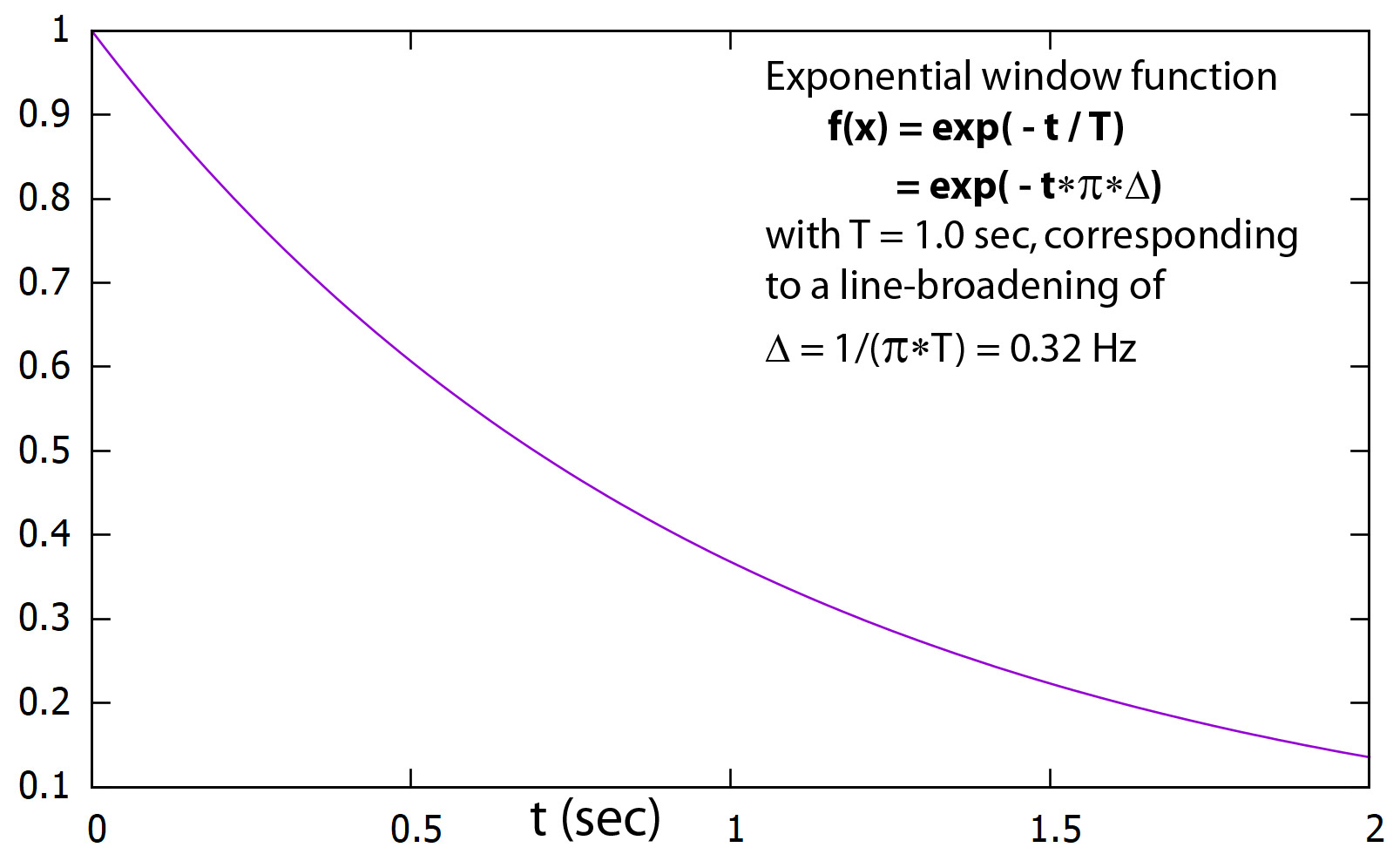
Steps Before FT: Window Function and Zero Filling

Window function to minimize truncation artifacts

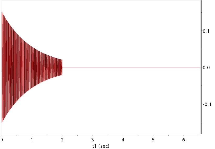
Original FID is zero-filled to 3 times of original size above.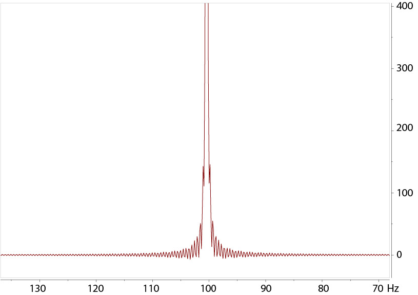

Truncation artifacts seen without window function before FT

Zero filling (ZF, appending zero-value data points to the FID) is almost always done before FT to give good digital resolution of the FT spectrum. Typical acquisition time of an FID for a small molecule is ~ 5X of the longest T2 among the spins. Often, 2-3 secs is adequate. ZF is often applied to at least double the original FID data size. Further zeros appended often only increase the smoothness of the spectrum without further gain in resolution.

A window function, also called apodizaton function, is used to smooth the FID to remove the sudden cutoff at the end of the FID so that the data drops to or close to zero intensity before ZF. Without the window function, the sharp ending of the signal causes base oscillation called truncation artifacts.

The figures above illustrate the impact of a simple window function of exponential decay curve multiplied to the FID, then zero filled to 3X data points followed by FT. The exponential function rate of decay corresponds to a line-broadening effect of 0.2, 0.5, and 1.0 Hz to the signal's natural broadness. With 0.2 Hz, a small amount of truncation artifacts are still visible at the base of the peak. A good balance here is 0.5 Hz, which removes the artifacts without broadening the signal further.

0.2-0.5 Hz is typical for small molecules with very sharp signals, given that the natural width is not much bigger than this range. For a naturally broad peak (such as those broadened by paramagnetic ions), a larger value should be used to smooth the signals from other noises in the spectrum.

Truncation Artifacts from Digital Overflow

The ADC board converts the FID analog signal into digital values, but it can only handles up to the maximum chip capability, 16-bits or 32-bits. On a 16-bit chip (2¹⁶ max range), the maximum, signed integers stored are ~ +/-32800. A proper gain for amplification should allow the maximum signals throughout the experiment to fit into this range. As the FID decays to smaller values over the detection, the beginning part of the FID often has the most danger to overflow. For simple 1D experiment, gain is set automatically. For arrayed experiments, however, the user needs to set a fixed gain before an experiments starts.

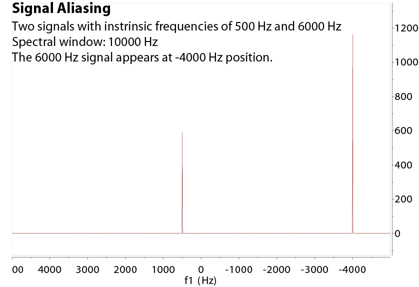
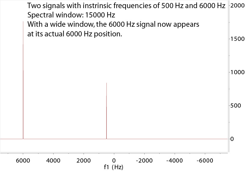
Signal Folding or Aliasing: Actual or Apparent Resonance Position?

There is no absolute signal frequency in the detected spectrum. This relativity, however, must be distinguished from the intrinsic resonance frequency of a nuclear spin that corresponds to the quantum energy difference of the up and down spin states in the given magnetic field. This frequency is absolute and is only relative (and linear) to the magnetic field strength. The detection process, however, necessarily uses a reference frequency and a limited bandwidth. These set up an interesting and often misleading apparent resonance shift position, through a signal "folding" or "aliasing" process. Signal aliasing is a widespread phenomenon. It is rooted in the limited, discrete resolution we can obtain in any detection. If we think about this, the quantum mechanical discreteness and quanta come naturally in the real world, much more obvious and natural than the mathematical continuity. This finite resolution in observation means that we essentially always observe with an aliasing filter.

When the resonance frequency is outside the detection window (centered at 0Hz), the signal in the FT spectrum is "aliased" or folded into the detection window by an equal distance from the opposite edge. This is equivalent to a translation of the signal by a full (or multiple) spectral window. In the time domain, this arises from the equivalence of sine or cosine functions with one or multiple phase shifts of 2π. This phenomenon is general called the Nyquist-Shannon sampling theorem.

As a matter of fact, the only reason we know the resonances are at their natural shift positions is from the knowledge of chemical shift spreads, consistency in the lock, and instrument clock reference frequency. The instrument itself sees no difference in the digitized signal between a peak and another shifted multiple spectral widths away in the direct detected dimension. For the indirect dimension in 2D-4D experiments, however, this frequency difference of one or multiple spectral width shifting can be differentiated to some degree and encoded neatly in the pulse sequence itself, through a delay, called half dwell-time delay. This delay, added to all increments in the 2nd dimension, effectively causes a 180-degree phase shift to the signals outside the detection window by an odd number of the window width. This leads to an opposite sign of the signals sitting outside by one (or 3, 5, ...) spectral windows. To do this trick in the direct dimension is complicated by the extra work that is needed to deal with linear phase correction. However, an easy test of window size change suffices and it is also true that for peaks way off the excitation center (center of spectrum), the signal intensity will get weaker and may be distorted as well.

Overall, care must be taken to interpret the "apparent" peak positions, especially for X-nuclei. If you have any doubt, a wider spectral window should be used and tested to make sure the resonances stay where they are, then the window should be set narrower for best data quality. If any peak moves upon a change of spectral window either bigger or smaller, it means it is folded from outside the window. However, do not use a huge spectral window because it sacrifices other spectral qualities, including distorted baseline and extra unfiltered noises.

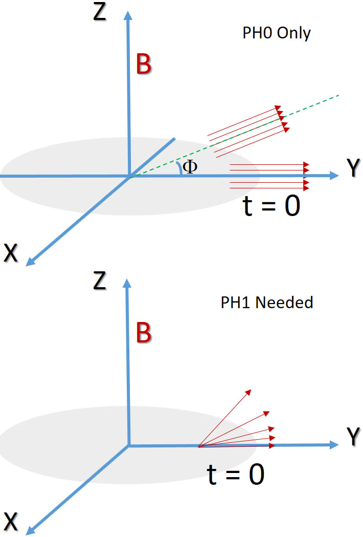
Phase Correction: Zero Order (PH0) and First Order (PH1)

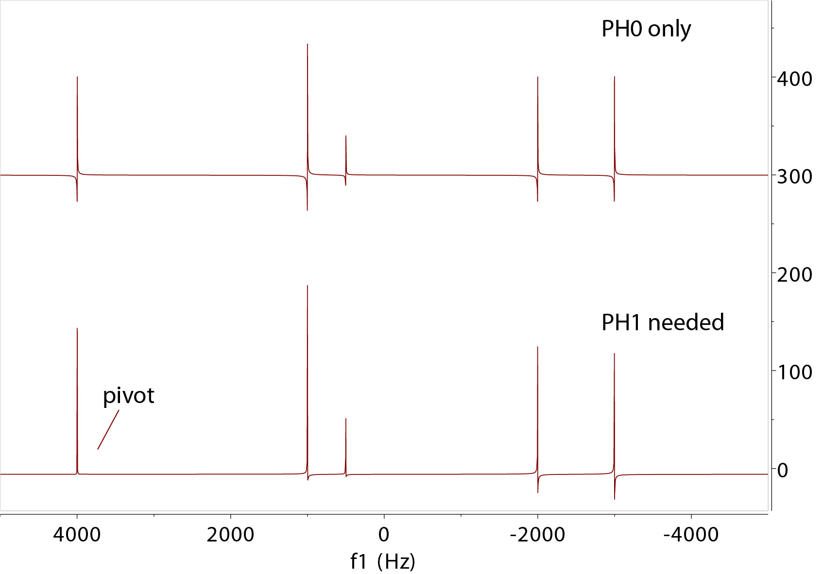
Zero (PH0) and First Order (PH1) Phasing

After FT, the spectrum has to be phased to pure "absorption" mode (pure up or down peaks). Phasing involves both zero-order and often first-order adjustment. Zero-order (PH0) phase is the same across the spectrum for all peaks. First-order (PH1) is applied to peaks by a linearly changing amount starting from a "pivot" point where the 1st-order phase adjustment is zero. You recognize the need for 1st order phase correction by observing the dissimilarity of the peak shape distortions across the spectrum from one side to the other.

You may pick any pivot point but it is often set at a strong peak on one side of the spectrum. The peak at the pivot point is adjusted for zero-order phase correction. Then, you may adjust the first-order phase correction that is applied to the rest of the peaks away from the pivot. The PH1 linearity guarantees what work for the extreme ends works for the middle peaks as well.

The right picture above depicts the cause of zero and 1st order phase correction. At the start of data collection, if all spins (each gives one ¹H peak) point to the +Y axis direction and therefore have the same phase, no phase correction is needed in the final spectrum. If at t=0, they point in the same direction but are rotated away from the Y axis by the same angle, they need a zero order phase adjustment corresponding to a rotatation back to the Y axis.

If at t=0, they have "dephased", which means they have fanned out with a spread angle caused by the frequency differences, then a 1st order phase correction with or without a zero order correction is needed. The 1st order correction will put the spins back to the same direction at t=0.

Dephasing of the spins at the start of acquisition can be caused by various delays in the pulse sequence and detection process. These imperfections can be compensated by reversing the extra delays in the pulse sequence but often a small amount of PH1 can be easily dealt with during processing.

Consider a signal at -5000 Hz and another at 5000 Hz. If they start in the same direction initially, a small 100 microsecond delay will cause the two signals to fan out an angle of 2πft=2*3.14*(5000+5000)*0.0001=6.28 degree. 1 msec delay causes an angle of 62.8 degree. This means if one signal is in-phase, the other will be off by 62.8 degree. This angle is adjusted back and removed in 1st order phasing.

Updated, Jan-Feb 2019, Hongjun Zhou