NMR Theory and Techniques
Note: During training and assisting students and researchers, I often find it helpful to go over some
NMR theory which is usually picked up in bits and pieces sporadically over the years for most users. Evidently, this work has evolved
into a much bigger project in a short time. I hope these materials will spur more interest in NMR and
help all users, especially new ones, to broaden their skills and understanding of the NMR techniques. Some
data shown here are synthesized, perfect data for illustration purposes. The data are generated with in-house
written Tcl/Tk scripts, converted to nmrPipe binary
data, and then processed with Mnova. Many common NMR terminologies are
highlighted in bold. Since other aspects of the NMR techniques are covered in various lab classes, focus is given here
to better understanding the mathematical and physical basis of various NMR observations and techniques.
Some are very relevant to routine practice, especially in the design of NMR experiments and data interpretation.
-- Hongjun Zhou, @UCSB, 01/2019
"I insist upon the view that 'all is waves'." -- Erwin Schrödinger in Letter to John Lighton Synge (1959)
Transient NOE
As shown above, steady-state NOE with spin saturation provides no information about the inter-atom distance
except that the atoms showing NOE are likely within 5 Å. Under saturated, steady-state condition,
the strength of NOE and the measured NOE enhancement factor are strongly influenced by various leakage relaxation pathways
and undesirable, indirect couplings through spin diffusion. It lacks details about the
closeness of the two atoms. While a single, high %NOE approaching the maximum (50%) indicates a very close distance,
a weak NOE and in some cases, the lack of it, doesn't reliably address the distance question at all
due to unknown leakage relaxations. This leakage from useful, one-to-one cross-relaxation may be from other
adjacent spins, 1H's in particular, or from other time-dependent
fluctuating perturbations to the two spins of interest, such as a small amount of paramagnetic ions in the sample.
A NOE buildup curve as a function of saturation time provides a way to get around the problem of lacking
a distance dependence in steady-state NOE, but it is inefficient.
In transient NOE measurement, the spins are left
along Z axis to relax during a mixing period of ~ 0.5 to 1.0 sec for small molecules
to allow cross relaxation to build up NOEs. Transient NOE measurement as
done in 2D NOESY (or its 1D analog) also suffers from leakage relaxation but overall it is a far better method of NOE measurement
in nearly all circumstances. It has the advantage of detecting all NOEs
between all 1H's at once
rather than doing so one at a time as in steady-state NOESY. The reliability of NOESY in distance assessment in a multi-proton
molecule relies strongly on the redundancy of inter-proton distance information which is difficult to obtain in selective saturation. We will consider
the distinction of these two types of NOE, the underlining relaxation
mechanisms in transient NOE, and the distinct dynamic regimes separating the NOE observations between
small and macro- molecules.
NOE Crosspeak and Diagonal Peak Intensities
In a NOESY experiment with a mixing time τm, the amplitudes of the diagonal (axial, aAA and aBB) and crosspeak
(aAB and aBA) intensities between
two like spins A and B (i.e. two 1H spins) are described in the following equations (S. Macura & R.R. Ernst, 1980):
aAA = aBB = (M0/2)*exp(- RL*τm)*[1 + exp(- RCτm)]
aAB = aBA = - (M0/2)*(W2 - W0)/|W2 - W0|*exp(- RLτm)*[1 - exp(- RCτm)]
with:
RC = 2|W2 - W0|,
RL = R1 + 2W1 + W0 + W2 - |W2 - W0|
Note the missing "-" sign typo error in aAB in the reference paper above which was corrected later in the book by Ernst et al (1987). M0
is the initial A and B population along Z at the beginning of the mixing period.
The transition rates take the forms:
W1 = (3/2)*q*J(ω)
W0 = q*J(0)
W2 = 6q*J(2ω)
with q = 0.1γA2γB2/r6ℏ2(μ0/4π)2
J(ω) = τc/(1 + (ωτc)2)
J(ω) is the reduced spectral density or transition density (per second); ω is the angular
frequency of the transition, here the Larmor
frequency of the spins (ωA ≈ ωB = ω) separated by distance r; τc is the rotational
correlation time of the molecule carrying the two spins.
RL is the leakage relaxation rate that doesn't lead to NOE crosspeaks while the cross-relaxation rate
RC gives rise to NOE. We can see RL
reduces both diagonal and NOE peak intensity by the same factor exp(- RL*τm). The ratio aAB/aAA,
therefore, is independent of RL.
Distinct NOEs Under Fast and Slow Motion
From the equations above, the observed NOEs fall under two different regimes with the dividing critical point at
W2 = W0 which leads to RC = 0 and zero NOE intensity. This corresponds to ωτc = √5/2 = 1.12.
At 600 MHz field, the critical τc is ~ 0.3 nsec; at 400 MHz, it is ~ 0.45 nsec. This
means that lower field may help small molecule NOEs at the sacrifice of NOE intensity from lowered sensitivity.
When W2 < W0,
the NOEs are positive, and the signs of aAB and aBA are the same as aAA and aBB,
leading to the same signs for NOE and the diagonal peaks.
When W2 > W0, the NOEs are negative, and the signs of the NOE crosspeaks and the diagonal peaks are
opposite. This separation corresponds to two motional regimes:
- Extreme narrowing or fast motion where ωτc << 1: this is for
small molecules with very fast tumbling time. J(ω) = J(2ω) = J(0) = τc. We have W2 > W0.
Negative NOEs are observed.
- Slow motion or spin diffusion limit where ωτc >> 1: this is for macromolecules with slow tumbling
time of τc >> 1 nsec. J(ω) = J(2ω) = 0, J(0) = τc. We have W2 < W0.
Positive NOEs are observed.
In between these two timescales, NOEs are very weak or absent.
Notably, 1/r6 scaling of the transient NOE intensity
is embedded in RC, a distinction from steady-state NOE. To see this relationship for fast motion,
we set ωτc = 0, then J(ω) = J(2ω) = τc, and W1 = (3/2)qτc,
W0 = qτc,
W2 = 6qτc. These give rise to:
RC = 10qτc, RL = R1 + 5qτc
for small molecules.
For two 1H spins separated by a distance of 4 Å, q = 1.39X10+7 sec-2. For a small molecule with
rotational correlation time τc << 1 nsec (10-9 sec), we have: qτc << 0.0139/sec or
RC << 0.139/sec. Typical T1 values
for small molecules are > 1 sec or R1 < 1. With a NOE mixing time of ~ 0.5 sec, we have
RCτm << 0.07. Using the approximation ex ≈ 1 + x for small x, the term "1 - exp(- RCτm)"
in aAB and aBA is reduced to RCτm ~ qτc ∝ 1/r6. Therefore,
aAB and aBA are proportional to 1/r6.
For macromolecules, ωτc >> 1, leading to J(ω) vanishing except for J(0). This leaves RC = 2W0 = 2qJ(0) = 2qτc.
With τc ~ 5 nsec (5X10⁻⁹ nsec) for a small protein molecule of ~ 60 residues, RC ~ 0.07/sec.
With a typical NOE mixing time of ~ 0.15 sec for macromolecules, we have RCτm ~ 0.01, and
aAB and aBA are again proportional to 1/r6.
Difference in Maximal Transient and Steady-State NOEs
First, we consider absolute NOE intensity. From aAB equation above, we have:
aAB ~ exp(- RLτm)*[1 - exp(- RCτm)]
To find the maximum aAB, we take the derivative of this term against τm:
daAB/dτm ~ - RL*exp(- RLτm) + (RL + RC)*exp(- (RL + RC)τm)
Setting daAB/dτm = 0 gives us:
RL = (RL + RC)*exp(- RCτm)
This leads to the ideal mixing time where NOE is at its maximum:
τm = (1/RC)*ln(1 + RC/RL)
Replacing the terms with τm with the optimal value, we obtain the maximum intensity
of aAB:
aAB = ±0.5M0*ρρ(1 + ρ)-(1+ρ)
where ρ = RL/RC. For small molecules, ignoring R1, ρ = 0.5 which leads to aAB = -0.19M0.
However, if the leakage R1 = 0.5RC, then ρ = 1, the NOE peak drops to aAB = -0.125M0
For macromolecules, RL = R1. Assuming the leakage rate R1 = RC, then ρ = 1,
leading to aAB = 0.25M0.
Similar estimates can be made with the following. For small molecules, if we ignore the leakage R1, we have the ideal mixing time for maximum NOE:
τm = 1/(10qτc)*ln(3) = 0.11/(qτc)
For a small molecule with τc ~ 0.2 nsec, qτc ~ 0.00278, the maximum NOE is achieved
at τm ~ 40 sec. With this mixing time,
the maximum NOE intensity is aAB ~ -0.19*M0, or ~ -19% of the initial magnetization or aAA
at τm = 0. This should be compared with ~50% maximum NOE under steady-state saturation.
However, with leakage
relaxation considered, the maximum NOE is achieved at much shorter mixing time. If R1 contributes
R1 = 5qτc, τm drops to ~ 25 sec when the maximum NOE is achieved. This
leads to a maximum NOE intensity of aAB ~ -0.125*M0 or ~ -12.5% of the initial magnetization or
aAA at τm = 0. Practically, leakage through other spins, the lattice and spin diffusion is
substantial. The mixing time is limited to < 1 sec. Therefore, the NOE intensities in both transient and steady-state measurements
are substantially weaker than the ideal cases.
Calculated NOE Values
The following figures show calculated NOE value as a fraction of initial spin magnetization M0 and
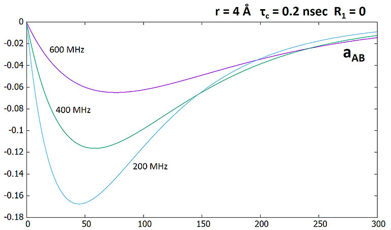
as a function of mixing time (sec). ωτc = 0.25, 0.5 and 0.75
at 200, 400 and 600 MHz field, respectively, except for the last figure. M0 is not scaled
by the field strength B. SNR is related to the field B as SNR ∝ B1.5. At
600 MHz, SNR is ~ 1.84 times of that at 400 MHz.
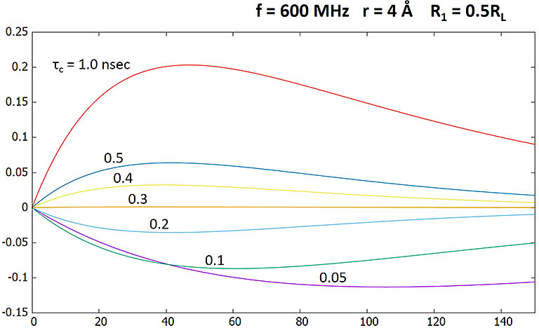
NOE Intensity (unit: M0) as a Function of Mixing Time (sec) |
|
NOE as a function of mixing time (sec) at different fields. Unit of NOE is M0. Although NOE is higher at
lower field as a proportion of initial magnetization, overall it loses due to lower sensitivity at lower field. SNR
at 600 MHz is ~ 84% higher than at 400 MHz.
|
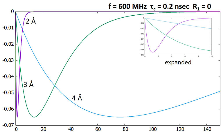
NOE as a function of mixing time (sec) with the two proton spins at different distances.
Sharp changes reflect 1/r6 dependence.
|
|
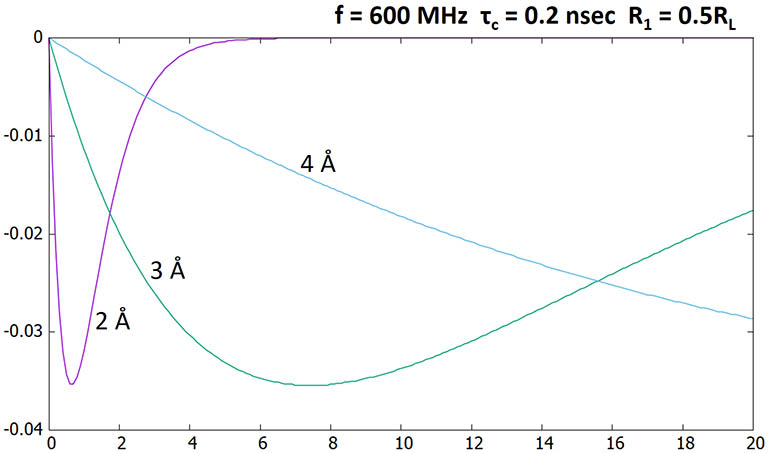
Here the leakage rate R1 is set to make up half of RL. NOE intensity drops by half. The optimal
mixing time also shortens by ~ half.
|
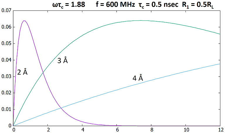
Here ωτc = 1.88, larger than the critical 1.12. Positive NOEs are produced.
|
NOE Relative to Diagonal Peak
Next, let's consider the relative intensity of the transient NOE peak over the diagonal peak.
Taking the ratio aAB/aAA, we have:
NOE = - [1 - exp(- RCτm)]/[1 + exp(- RCτm)]
For fast motions, RCτm and RLτm are small (see above), leading to the approximation:
NOE ≈ - RCτm/(2 - RCτm) ≈ - 0.5*RCτm
When the mixing time is short so that RCτm << 1, the NOE ratio with the diagonal peak is linear with τm. With a typical mixing time
of 0.5 sec, the NOE is ~ - 3.5% of the diagonal peak intensity for the 1H spin pair above. It is notable again
that the ratio of the transient NOE peak with the diagonal peak is proportional to 1/r6 which is embedded in RC.
NOE Intensity (unit: M0) as a Function of Mixing Time (sec) |
|
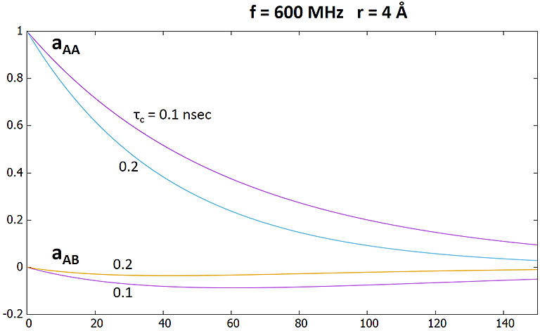
NOEs under different rotational correlation time are compared. Negative NOE is limited
in magnitude. Positive NOE increases dramatically as τc increases. |
Compare NOE amplitude aAB with the diagonal peak aAA. |
The NOE to diagonal peak intensity ratio aAB/aAA
is independent of RL, removing most of the variable dependence on auto- and leakage relaxation. It can be used to more
accurately measure the distance between atom pairs if
a reference pair of protons and their distance and ratio of NOE over diagonal peaks are compared with and scaled with 1/r6. This
is commonly done in biomolecular NMR studies during calibration or classification of
inter-atomic distances based on hundreds to thousands of observed NOE crosspeaks to be used as distance constraints in structural computation.
In summary, although transient NOE is weaker than steady-state NOE, its 1/r6 dependence is highly desirable and allows
comparison of NOE intensities between different atom pairs in the same 2D experiment to extract more accurate distance information.
The set of distances with a degree of redundancy can then be used more reliably to infer structural details of the molecule in the presence
of unknown leakage relaxation.
With steady-state NOE measurement, this is not possible or feasible; its use
in structure elucidation, especially with NOE difference experiment (CYCLENOE) to infer distances
based on quantitative %NOE is not justified in most cases.
References
- S. Macura & R.R. Ernst (1980). Elucidation of cross relaxation in liquids by two-dimensional NMR spectroscopy, Mol. Phys. 41, pp. 95-117.
- R. Ernst, G. Bodenhausen and A. Wokaun. (1987) Principles of Nuclear Magnetic Resonance in One and Two Dimensions.
Updated, Jan-Feb 2019, Hongjun Zhou
©2019 The Regents of the University of California. All Rights Reserved. UC Santa Barbara, Santa Barbara, CA 93106