NMR Theory, UCSB Chem and Biochem NMR Facility

NMR Theory and Techniques

Note: During training and assisting students and researchers, I often find it helpful to go over some NMR theory which is usually picked up in bits and pieces sporadically over the years for most users. Evidently, this work has evolved into a much bigger project in a short time. I hope these materials will spur more interest in NMR and help all users, especially new ones, to broaden their skills and understanding of the NMR techniques. Some data shown here are synthesized, perfect data for illustration purposes. The data are generated with in-house written Tcl/Tk scripts, converted to nmrPipe binary data, and then processed with Mnova. Many common NMR terminologies are highlighted in bold. Since other aspects of the NMR techniques are covered in various lab classes, focus is given here to better understanding the mathematical and physical basis of various NMR observations and techniques. Some are very relevant to routine practice, especially in the design of NMR experiments and data interpretation. -- Hongjun Zhou, @UCSB, 01/2019

"I insist upon the view that 'all is waves'."
-- Erwin Schrödinger in Letter to John Lighton Synge (1959)

Transient NOESY: A Better Method of Measuring NOEs

Pulsed Field Gradients (PFG): Now You See It, Now You Don't

Gradient Shimming

Shimming is a process of adjusting shims to bring the field to uniformity along Z and to minimize any fields in the XY plane over the sample area. Manual shimming to achieve sharp signals is often a tedious process if the starting points are far off. Gradient shimming is undoubtedly one of the most useful and time-saving routine tools on a modern NMR spectrometer. Without it, a user would spend more time on shimming than actually collecting a simple ¹H spectrum, and many automated data collection features would be impossible.

Gradient shimming was proposed in 1994, borrowing the idea of gradient imaging, by P.C. van Zijl, S. Sukumar, M. O'Neil Johnson, P. Webb, R.E. Hurd, Optimized shimming for high resolution NMR using three-dimensional image-based field mapping, J. Magn. Reson. A 111 (1994) 203-207. The method itself is quite simple, in fact, and can be used with X, Y, and Z gradients with little change. Of note, shims are gradients as well, and are designed to have various shapes of harmonic functions of X, Y and Z coordinates. Z1 shim is designed to be a linear gradient. Pulsed Field Gradient (PFG) is used here as a stronger, independent gradient pulse with known good linearity, but gradient shimming can also be done with Z1 gradient, also called "homospoil" (homogeneity spoil) gradient, in place of PFG.

The solution has three parts: (1) measure B field deviation in a sample as a function of Z, (2) map the individual shim profile as a function of Z (or X, Y, Z in 3D shimming along all axes), and (3) use the shim profiles and apply the right shim changes to remove the field inhomogeneity. Here we only discuss Z-gradient shimming but the method equally applies to XY shimming. As in imaging, gradient pulses are used to encode the spins by their Z axial positions. The field deviation is simply an additional, small gradient term that has to be extracted.

If the B_z field deviates from a constant value B₀ by ΔB, the phase accumulation under a shim G_i(z) gradient of duration d₃ is:

Δφ(z) = γ(G_i(z) + ΔB(z))*d₃ (1)

where G_i represents the gradient strength of one of the shims (i.e. Z1, Z2, etc) at position z. With PFG on during acquisition, a spectrum with this phase change is a wide-spread signal with the frequency encoding the Z axial position of the spins. Δφ(z) is calculated by the real and imaginary parts of the data at each Z position (each frequency data point) encoded in the frequency. However, to extract ΔB(z), each individual shim profile G_i or simply an offset from a constant level, ΔG_i, has to be known.

We can see that by varying G_i by dG, through the difference in Δφ, we are able to cancel the unknown field inhomogeneity ΔB in (1) and obtain the G_i profile along Z:

Δ(Δφ)(z) = γdG_i(z)d₃ (2)

Generating the shim profile, called a shim map of the probe, is the first step of gradient shimming. This is usually done with a separate sample and the profile is saved for shared use. The following gradient shimming pulse sequence is designed to map the shim profiles.

Varian's Gradient Shimming Pulse Sequence
TOP

Here d₂ = 1 msec. Acquisition time at is ~ 2.5 msec for ¹H and ~ 17 msec for ²H shimming. G_z is PFG used to spatially encode spins along Z. dG represents the combined shims or simply the change of one shim gradient as the experiment is designed to do with each detection. For each shim change, d₃ is arrayed, set to 0 and a ~ 5-10 msec delay, and a spectrum is acquired with each shim setting, Z1 to Z5. With all other pulses and delays being equal, the difference between the two spectra collected with the two d₃ values gives Δ(Δφ(z)) = γdG(z)*d₃ for each shim. The dG_z curves are the shim map of the probe.

The goal of shimming is to remove ΔB across the sample area with changes in the shim coils. Once dG_i(z) or the shim profiles for Z1, Z2, Z3 .. etc. are known, they are combined to remove ΔB(z) measured separately during each gradient shimming routine. The detection nucleus is usually deuteron from deuterated solvent, but ¹H works well for samples in H₂O due to its intense signal or in a situation where ²H signal is weak or absent from the sample.

Shim map Created with ²H Detection. The sample has 99% D₂O with 1% H₂O. Each shim, Z1 to Z5, has a unique shape that is designed to give a field shape of an independent, specific order of harmonic function. The actual profile of each shim as a function of Z (freqency encoded horizontal axis) is measured with the method in the right figure.

Mapping the shim profiles of Z1 to Z5. The shim values are varied with ~ 1000 DAC unit change within each pair of curves, from Z1 to Z5, starting from current shims. The first and last pairs of curves are using the current shim values. Within each pair, the delay d3 is varied from zero to a set value (~ 250 msec here). The difference between the two curves gives the profile of the shim that is varied within the pair according to equation (2) above.

The differences between the pairs are not obvious because it is the phase of the time-domain data that is extracted to give the individual shim profiles on the left (see equations 1-2 above). The plots shown during Varian's mapping protocol are obviously in magnitude mode that removes the phase data.

Autoshim Fitting
TOP

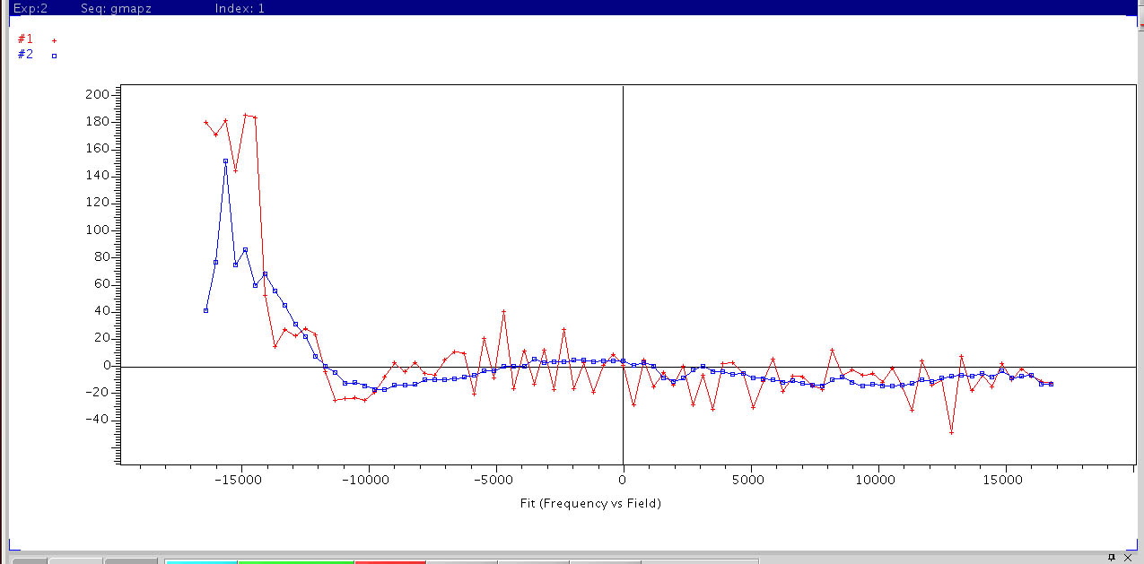Autoshim on Z. During autoshimming, a linear combination of changes in Z1 to Z5 are applied according to the shim profile curves with the goal of removing field variations across the sample area. Shown above are the detected field maps of the last two iterative fittings which have converged to meet a target criteria. The vertical axis is the calculated field variation in Hz. The horizontal axis is the position encoded frequency along Z in Hz with the center of the NMR tube at 0 Hz.

Updated, Jan-Feb 2019, Hongjun Zhou