NMR Theory, UCSB Chem and Biochem NMR Facility

NMR Theory and Techniques

Note: During training and assisting students and researchers, I often find it helpful to go over some NMR theory which is usually picked up in bits and pieces sporadically over the years for most users. Evidently, this work has evolved into a much bigger project in a short time. I hope these materials will spur more interest in NMR and help all users, especially new ones, to broaden their skills and understanding of the NMR techniques. Some data shown here are synthesized, perfect data for illustration purposes. The data are generated with in-house written Tcl/Tk scripts, converted to nmrPipe binary data, and then processed with Mnova. Many common NMR terminologies are highlighted in bold. Since other aspects of the NMR techniques are covered in various lab classes, focus is given here to better understanding the mathematical and physical basis of various NMR observations and techniques. Some are very relevant to routine practice, especially in the design of NMR experiments and data interpretation. -- Hongjun Zhou, @UCSB, 01/2019

"I insist upon the view that 'all is waves'."
-- Erwin Schrödinger in Letter to John Lighton Synge (1959)

Transient NOESY: A Better Method of Measuring NOEs

Pulsed Field Gradients (PFG): Now You See It, Now You Don't

Pulsed Field Gradients (PFG): Now You See It, Now You Don't

Pulsed Field Gradients play a ubiquitous, important role in modern NMR pulse sequences. Magnetic field gradient is key to Magnetic Resonance Imaging (MRI), a non-invasive diagnostic technique widely used in the medical field. MRI uses spatial encoding with field gradients to obtain a 3D image of the spin density, such as ¹H density, according to their location and relaxation properties. The density map weighted by different spin properties, such as relaxation rates, often differentiates among different cell and tissue types and may be used to identify tumor, for example. Initially, this technique was called 'Zeugmatography' by P. C. Lauterbur at SUNY Stony Brook in 1973 who first obtained 2D images of glass capillaries of H₂O:

"Because the interaction may be regarded as a coupling of the two fields by the object, I propose that image formation by this technique be known as zeugmatography, from the Greek ζενγμα, 'that which is used for joining'." (P.C Lauterbur, (1973) Nature 142, 190).

Paul C Lauterbur along with Peter Mansfield was awarded the Nobel Prize in Physiology or Medicine in 2003 for the development of MRI techniques.

A magnetic field gradient allows NMR observation to be highly tunable, selective, and targeted. In high-resolution NMR, its well-known applications include gradient-aided shimming and Diffusion Ordered Spectroscopy (DOSY). Here we focus most of the discussion on the common use of Z-axial PFG in high-resolution solution-state NMR studies which serve very different purposes from MRI. Gradients along X and Y axes play similar roles and follow similar principles. PFG can be used to briefly (~50 micro seconds to a few msecs) spoil the magnetic field homogeneity (uniformity) across the sample area in a controlled and often reversible fashion. It can be used to destroy unwanted magnetizations or coherences, select coherence by its order, or to dephase signals temporarily and refocus them back at a later point, or to code the spin procession frequencies according to its Z-axis position in the sample and vice versa.

Two related consequences are brought by a Z-axis gradient field: (1) if acquisition is in the presence of a field gradient, it causes a position-dependent change of resonance frequency and therefore relating the frequency with position, a phenomenon called spatial encoding; and (2) if the signals are allowed to evolve under Z-gradient followed by gradient-free detection, a position dependent phase accumulation occurs. This is called phase encoding. Both are often linear with the sample slice position along Z and are based upon the same physical origin.

Spatial Encoding

Spatial Encoding with Active PFG During Detection

Magnitude-mode Imaging reflecting spread of linear field along Z

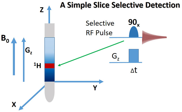
A selective, shaped RF pulse can be applied simultaneously with a gradient pulse (G_z) to flip the spins in a frequency band spatially encoded by the gradient pulse to the XY plane for detection. Spins in other regions are left untouched along Z, the static field B₀ direction and their signals are effectively filtered out. An X or Y, instead of Z axial gradient can be similarly applied, creating a vertically cut slice selection with its plane perpendicular to Y- or X- axis.

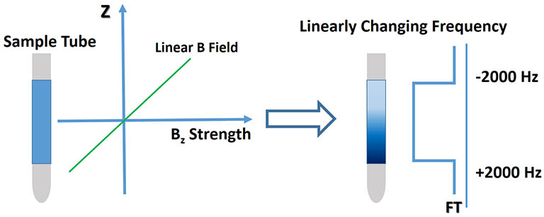
Shown above is an illustration of the effect of a field gradient. Once applied, it creates an additional, linear B_z field on top of the uniform static field across the sample area. This creates a linear resonance frequency encoding with ω = γB_z for the detected nuclei according to their Z-axis position. If the signal is detected with a wide bandwidth while the gradient is active and transformed in the magnitude mode, the NMR spectrum is a square-shaped spread of a signal with the high and low frequency given by molecules from the top and bottom of the sample area, a spatial encoding phenomenon. The intensity at each frequency is from a slice of the sample tube along Z, uniformly distributed as long as the sample concentration is uniform across the RF active region. In magnitude mode, the signal phase is removed (magnitude = (real² + imaginary²))^1/2) and only the amplitude or intensity of the signal is retained to avoid the need for phasing. This spatial signal separation technique is commonly used in imaging and gradient shimming. More selective RF pulses can be used to target a "band" of frequency (a physical slice of the sample under gradient) for manipulation or detection, potentially creating a useful technique for interesting slice-selective diffusion and scanning NMR experiments.

A gradient pulse typically lasts 50 microseconds to a few msecs, depending on gradient strength. It may then be turned off to allow other NMR techniques to proceed. Typical maximum strength of the PFG is ~ 80 Gauss/cm for a high-resolution solution-state NMR spectrometer and probe. It could be much stronger for more specialized use in imaging or solid-state NMR work.

To get an idea about what 80 Gauss/cm can do, let's consider how wide it can spread a ¹H signal in a typical RF region of 1.6 cm tall in an NMR tube. The gradient gives us an extra field spread ΔB_z = 80 Gauss/cm*1.6 cm = 128 Gauss. To translate this to frequency in Hz, simply multiply it by the γ of ¹H and divide it by 2π. We have Δf = γ_H*ΔB/(2π) = .... or easier yet, we simply take the field strength of a 500 MHz (¹H frequency) instrument at ~11.764 Tesla, and do a conversion. 128 Guass is 0.0128 Tesla. This gives us a frequency spread for a ¹H signal of: Δf = 0.0128/11.764*500E+6 Hz = 5.44E+5 Hz or 544 kHz. Only a strong NMR signal, such as ¹H from water at 110 M, can possibly survive this stretching. However, with such a wide spread in frequency, selective excitation of a frequency band under a strong gradient as shown in the figure above can be used to detect signals from a vertical slice of the sample.

With a dramatic simplification of the problem, to estimate the detectability of ¹H from water in MRI, let's assume we can easily detect 1 mM water ¹H with a single scan and a signal-to-noise ratio (SNR) of 10. At 110 M, the SNR would be 1.1 X 10⁶. Assuming a linewidth of ~ 1 Hz, spreading this water signal over 544 kHz means a SNR of ~ 1100/544 ~ 2 in the presence of the maximum gradient. This is a small signal but still observable. Typical PFG strength in use is much lower. Currently, the maximum gradient used in MRI is < 50 mT/m, or 5 Gauss/cm, about 15 times weaker than the maximum used in high-resolution NMR studies. With a 5 Gauss/cm gradient, the frequency spread is ~ 34 kHz. The narrower spread boosts SNR to 544/34*2 = 32, a highly detectable ¹H signal. With a larger volume of water content and faster signal relaxation expected from tissue materials, the ¹H SNR should be very good. These rough estimates show why MRI is able to use ¹H signal to image slices of body tissues. SNR for current MRI instruments ranging from 1.5T to 3.0T reaches 40-100 up to several hundreds in a typical imaging scan.

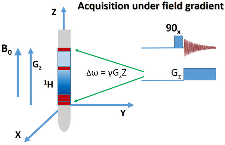
Spatial Encoding of NMR Signals Under Field Gradient
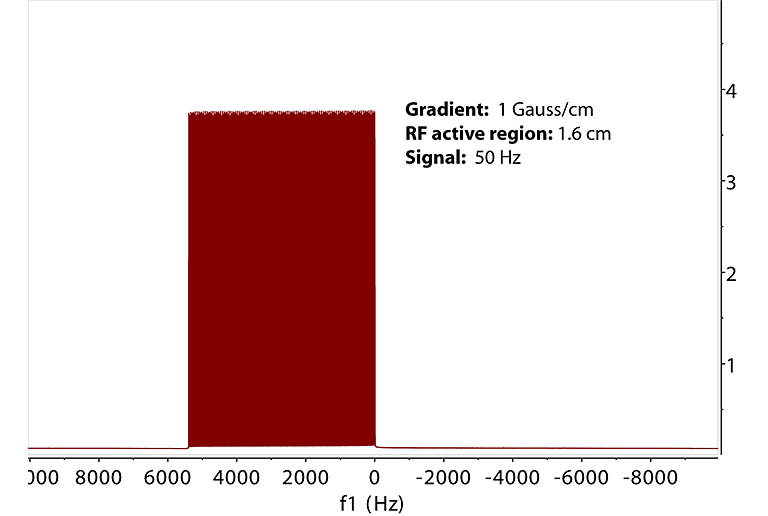
A. Acquisition under Z-axial field gradient G_z encodes the spin position with its resonance frequency. For illustration purpose, the sample is split into slices shown as filled red rectangles in the NMR tube. Spins from each slice resonate at a different frequency. The 90-degree RF pulse here is a hard pulse that excites spins over a broad bandwidth.	B. Spectrum acquired under field gradient. In this simulation, the RF active region of the NMR tube is split into 200 slices. A resonance at 50 Hz from a spin is now encoded by a slice-dependent shift in frequency afforded by the field gradient during acquisition. The field increases linearly from the bottom of the RF active region. In the FT spectrum, the single signal spreads over 5000 Hz. The low and high frequency corresponds to the bottom and top of the RF active region, respectively, if the field gradient is positive.
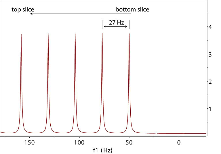
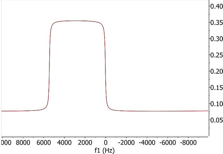
C. Expansion of the frequency region in B shows a signal from each slice equally spaced at 27 Hz which corresponds to the gradient encoding of 27 Hz shift from each slice of 0.08 mm thickness along Z. As the slice is cut thinner to approach continuity, the peak spacing gets smaller which leads to D.	D. Practically, the spin density and frequency shift are continuous which can be treated as a large line broadening effect for each slice. Applying a 100 Hz line broadening to mimic this continuity brings back a familiar spectrum seen during gradient shimming. Perfect linearity of the field gradient should give a flat and straight square intensity curve corresponding to equal spin population and broadness of signals in each slice.

Several important aspects about gradient pulses: (1) unless the gradient is present during acquisition, Z-axis PFG dephases signals in the XY plane and have no impact on the magnetizations along Z axis. (2) In a typical high-resolution NMR experiment, acquisition is done with the field gradient OFF except during gradient shimming. Thus, the frequency encoding in acquisition doesn't occur. The use of PFG in high-resolution NMR is predominantly in manipulating the signal phase rather than the position-encoded frequency detection. (3) Frequency or phase encoding with Z (or X, Y) gradient results from the same mechanism. The distinction is if gradient is present during detection.

Phase Memory and Encoding with Z-gradient

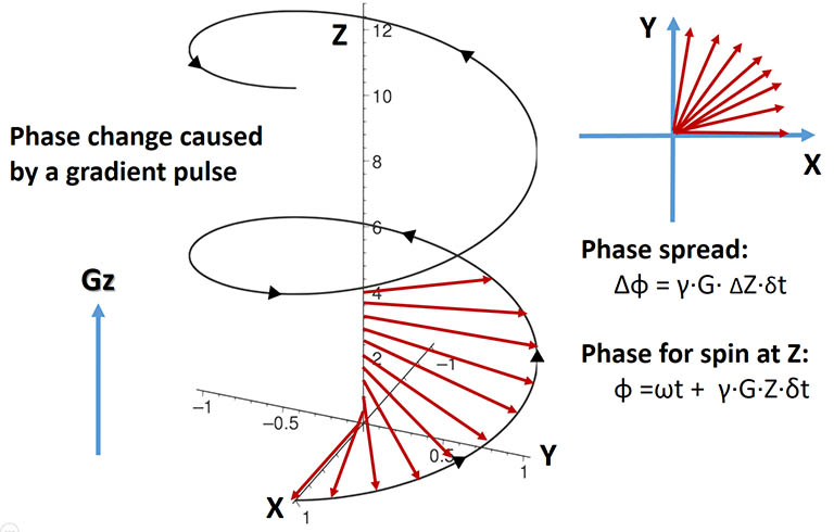
The picture above depicts an ensemble of spins in the RF active region rotating with a frequency ω, initially aligned along X. If a brief linear gradient pulse is applied for a duration of δt and turned off, the spins fan out in XY plane by a total phase spread: Δφ = γ*G*ΔZ*δt where ΔZ is the length of the RF active (detection) region, G is the gradient strength, and δt is the gradient duration. With sufficient G and δt, the collective signal from all spins may add up to zero intensity due to the phase variation across the sample. This is one of the main purposes of a gradient pulse, that is, to destruct an undesirable spin magnetization.

Dephasing NMR Signals by Field Gradient

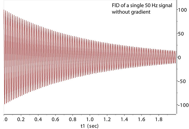
Gradient free FID. Its relaxation time T₂ is 1 sec.

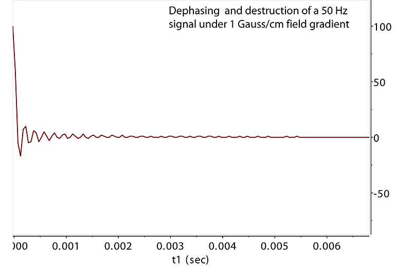
The 50 Hz signal is dephased in the XY plane across the sample area under PFG for duration t1, leading to signal destruction after ~ 5 msec. This technique, sometimes called homospoil when using Z1 shim instead of PFG, is widely used to remove unwanted coherent signals in XY plane. However, dephasing under PFG is a defined, "coherent" dephasing, not a random dephasing. The destructed coherence can be brought back alive before diffusion randomizes it spatially.

However, the position dependent extra phase is "memorized" and retained by the spins and lasts until translational diffusion destroys it when spins mix from different positions over time. DOSY is designed to measure the decay of this memory as a function of diffusion time and use the extracted diffusion parameters to gain insight into the size and shape of the molecule. It is also used to separate NMR signals in a 2D fashion for molecules with different diffusion rates.

Recover PFG-Dephased Signal
TOP

A single NMR signal is at 0 Hz. After the signal (I_x, I_y from all Z-axial slices) is dephased in the XY plane, another PFG is able to revive the lost signal if it is applied with a reverse sign and the same duration and strength, or different strength and duration combination as long as G_zΔt remains the same. This reversal effectively cancels earlier phase changes for all spins and brings them back into coherence. 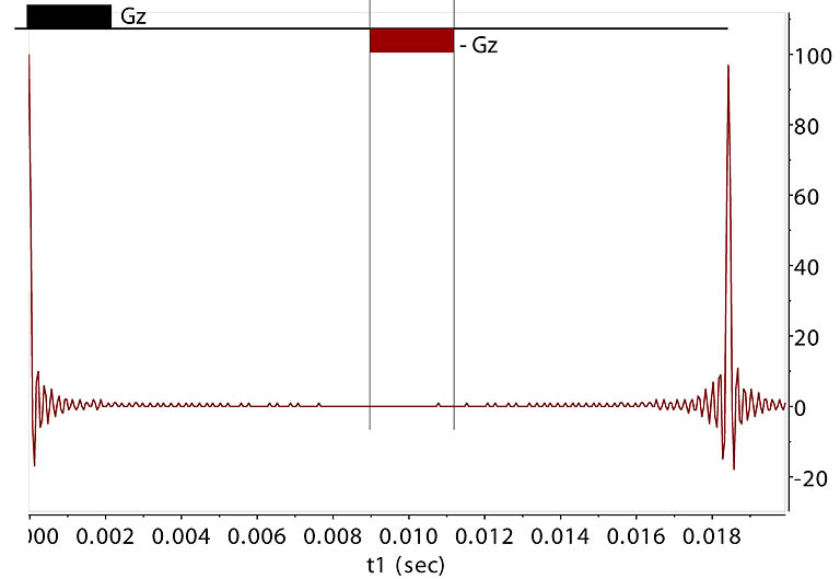The extent of this recovery is limited by the diffusion rate and relaxation. Here a 1 Gauss/cm PFG destroys the signal intensity within ~ 5 msec. A negative, 1 Gauss/cm PFG is applied, enabling coherence refocusing at an equal delay from the prior gradient pulse, creating an echo.

PFG is often used to selectively encode one type of spins by leaving them in the XY plane to be affected by the gradient while others are left on the Z direction and not affected. Dephased and encoded spins can be "refocused" and retrieved via a reverse gradient pulse, called a "refocusing" pulse. To do this for the spins above in the XY plane, we can simply apply a negative gradient of equal strength and duration, effectively canceling the earlier phase accumulation whatever the amount may be, as shown above. Adding a 180 RF degree pulse in the middle of spin procession removes the chemical shift evolution before detection. However, the 180 pulse reverses the front and back runners resulting from the first gradient, the refocusing gradient now needs to be the same sign as the first with the same phase accumulation (same γG_zδt) which can be achieved with the same G_z and duration. This is a simple gradient spin echo.

Coherence Selection

Coherence selection is another common use of PFG. This method is often quicker and avoids the phase cycling method which requires more scans to remove unwanted coherences and artifacts. If a coherence is expressed as the complex, circular polarization form, I_x, I_y are simply linear combinations of the left- and right- rotating coherences I⁺ and I^-:

I⁺ = I_x + i I_y, I^- = I_x - i I_y

A gradient pulse G_z lasting δt adds an extra phase to spins localized at Z:

I⁺ → I⁺e^-iγG_zZδt, I^- → I^-e^+iγG_zZδt

Now it is obvious that applying another gradient of opposite sign cancels the extra phase in the single quantum coherence. This cancelation also happens to double quantum coherences like I₁⁺I₂⁺ or I₁^-I₂^- involving two spins. However, for zero quantum coherences of like spins (with the same γ's), I₁⁺I₂^- or I₁^-I₂⁺, the field gradient has no impact because there is no extra phase addition under a PFG due to the opposite signs of the two phases, and therefore they are not destructed by a PFG. For unlike spins, i.e. ¹H and ¹⁵N spins, the situation is different. Under the gradient:

I⁺S^- → I⁺S^-e^{-i(γ_I - γ_S)G_zZδt}

The phase addition can be reversed as usual. More interestingly, for a specific coherence selection of this type, the phase additions for the two spins can be done under two separate gradients to avoid a total phase accumulation while other coherences are left with phase changes to be destructed. For the I and S spins, with two separate PFGs, we can achieve:

I⁺S^- → I⁺S^-e^{-i(γ_IG_z1δt₁Z - γ_SG_z2δt₂Z)}

For a ¹H and ¹⁵N spin pair, γ_H = -10γ_N. The two gradient strength and durations can be adjusted in such a way so that γ_IG_z1δt₁ = γ_SG_z2δt₂, the net phase addition is zero. This allows I⁺S^- and I^-S⁺ coherences to survive the second gradient while other coherences are destructed. This coherence selection is used in some HSQC pulse sequences and especially in sequences that need rapid data collection and a short phase cycle. PFG coherence selection can be done similarly to other orders of coherences and allows PFGs to play the magic of hide-and-seek.

Updated, Jan-Feb 2019, Hongjun Zhou