NMR Theory, UCSB Chem and Biochem NMR Facility

NMR Theory and Techniques

Note: During training and assisting students and researchers, I often find it helpful to go over some NMR theory which is usually picked up in bits and pieces sporadically over the years for most users. Evidently, this work has evolved into a much bigger project in a short time. I hope these materials will spur more interest in NMR and help all users, especially new ones, to broaden their skills and understanding of the NMR techniques. Some data shown here are synthesized, perfect data for illustration purposes. The data are generated with in-house written Tcl/Tk scripts, converted to nmrPipe binary data, and then processed with Mnova. Many common NMR terminologies are highlighted in bold. Since other aspects of the NMR techniques are covered in various lab classes, focus is given here to better understanding the mathematical and physical basis of various NMR observations and techniques. Some are very relevant to routine practice, especially in the design of NMR experiments and data interpretation. -- Hongjun Zhou, @UCSB, 01/2019

"I insist upon the view that 'all is waves'."
-- Erwin Schrödinger in Letter to John Lighton Synge (1959)

Transient NOESY: A Better Method of Measuring NOEs

Pulsed Field Gradients (PFG): Now You See It, Now You Don't

Magnetization and Coherence

NMR is fundamentally a quantum physical phenomenon. However, a significant portion of NMR can be described and understood qualitatively with a semi-classical physics picture. Without an external magnetic field, a diamagnetic material carries no net polarization, the nuclear spins point to random directions, and the magnetization is zero. In a strong magnetic field, these spins start to overcome thermal randomness and show a small degree of alignment along or in the opposite direction of the external field, giving a net magnetization. The alignment direction depends on the sign of the gyromagnetic ratio (see below).

At the atomic level, the up and down quantum states of a spin 1/2 nucleus carry a small energy difference allowing the lower energy state to be populated slightly more than the other (Zeeman Effect) according to the Boltzmann distribution. The Zeeman Energy is:

E = - μB = - γIB

where μ is the magnetic moment, B is the magnetic field, γ is gyromagnetic ratio (also called magnetogyric ratio), and I is the spin (angular momentum) operator. When the field is along the Z-axis, the equation is reduced to:

E = - μ_zB_z = - γI_zB_z = - ωB_z

where the last term ω = 2πf = γI_z is the corresponding resonant Larmor frequency. With currently available high-field superconducting magnets, this energy difference for a ¹H nuclear spin is on the order of the energy of a photon with the frequency (f) in the radio frequency (RF) range, a few hundred MHz to low GHz.

It comes naturally that sending in an RF wave to a sample sitting in the high-field magnet will excite some spins at the lower energy levels to the higher levels, given that the RF photon energy is around the energy difference between the spin states, or we may say that the nuclear spins will absorb the RF photons and jump into the higher energy states; any excess upper energy state spins may equally emit photons and come down to the lower states. The RF field may interact with the quantum states and cause the spins to be go between its eigenstates in a "coherent" manner. Spin manipulations through their interaction with RF pulses and time evolution of the quantum system is the core of NMR techniques.

A coherence in NMR is a physical state when many spins line up and rotate with the same speed around the magnetic field direction in the classical sense. Quantum mechanically, a coherence is a state where the spins oscillate between the different energy states (eigenstates) "constructively" (together with the same speed or phase). The counterpart of a coherence is spin "population" that refers to the spin populations in the "eigenstates" (spin up or down states for 1/2 spins).

To create a coherence, using a classical picture, we start from the polarized spins (i.e. I_z) and rotate them with an RF pulse into the XY plane, turning I_z into I_y and I_x terms. These X and Y components and the cross-products with them (i.e. I_zI_x, I_xI_y) are various orders of "coherences". The most commonly used technique involves the creation of single quantum coherence, such as ~ S_y (in-phase), I_zS_y (anti-phase) (or I_zS_x), through J-coupling. The single quantum in-phase and anti-phase types of coherences are the only observable ones. Others, not directly observable, are double quantum coherence (DQ) of the form, such as I_xI_y or I_1xI_2y for two separate spins. The correlated cross-products are used to correlate coupled spins in the indirect dimension in 2D double quantum filtered COSY (DQ-COSY), for example. DQ filtering removes correlations involving one spin or more than two spins.

Single Quantum Coherence, J-coupling

Simply speaking, a classical picture of a single spin rotating in the XY plane around the Z-axis magnetic field is a single quantum state and the simplest coherence. This coherence gives an NMR signal at the frequency of rotation.

More interesting, however, are spin-spin correlations that can be probed to provide structural information. A heteronuclear single quantum coherence (HSQC) experiment correlates two types of spins, i.e., ¹H and ¹³C through their through-bond coupling (also called J-coupling, indirect coupling, or scalar coupling) mediated by the surrounding electrons. This coupling is small relative to the Zeeman energy (compare ¹H-¹³C one bond J-coupling of ~150 Hz with a field strength of 600 MHz for ¹H or 125 MHz for ¹³C). The quantum perturbation theory generally works well here that allows the construction of the system states (¹H-¹³C spin system) from the eigenstates of isolated ¹H and ¹³C spins.

The spins have X, Y and Z components. Fortunately, for solution-state NMR, the situation is much simpler due to the fact that fast random molecular rotations randomize and cancel any XY components of the through-bond interaction to the first-order approximation, leaving only a coupling along Z-axis, with an energy contribution of:

ΔH ~ 2πJI_zS_z

where I_z and S_z are the Z-components of the nuclear spins of ¹H and ¹³C. This extra term commutes with the main Hamiltonian (quantum operator for energy which also has only Z spin components) and therefore simply contributes an extra energy of ±πJS_z for the S_z spin depending on the I_z values of ±1/2.

Given the main energy term for S comes in as 2πfS_z where f is the resonance frequency, the combined energy is now:

2πfS_z ± πJS_z = 2π(f ± J/2)S_z

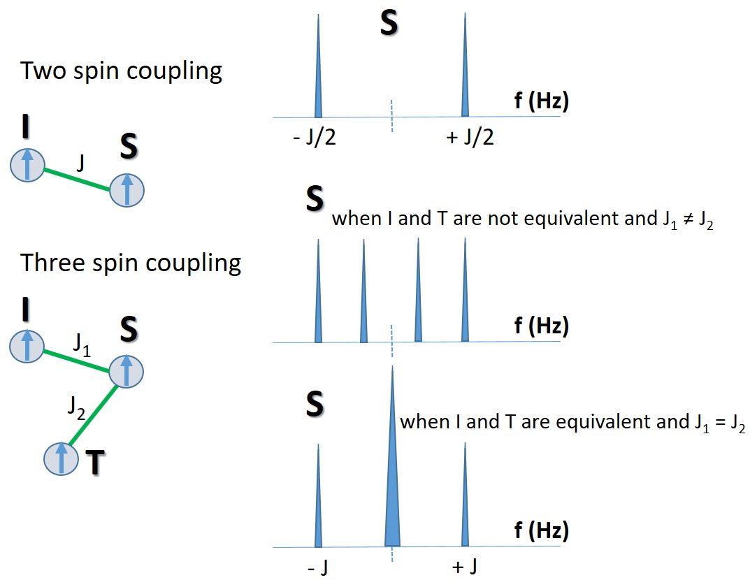
Therefore, J-coupling simply adds or subtracts πJ from the main energy term, leading to a splitting of J of the original resonance.

The two spin coupling Hamiltonian, 2πJI_zS_z, plays a very important role in the design of many NMR experiments, and it is also the simplest correlation to examine. The same theory applies to two through-bond coupled, unlike (means not from two indistinguishable ¹H's such as in a methyl CH₃ group) ¹H spins as well. In all the examples discussed here, the theory applies to any small J-coupling and whether it's one-bond, two-bond, and multiple bond J-coupling is irrelevant.

Through-bond Coupling Among More Spins

Nuclear spins interact with surrounding spins via the electronic cloud of the chemical bonds. Using the approach above, we can see how the resonance splits if the spin S (i.e. one ¹H) couples to two different and nonequivalent spins (i.e. protons I and T).

The extra energy affecting S spin is:

ΔE = 2πJ₁I_zS_z + 2πJ₂T_zS_z

With I_z and T_z each take either -1/2 or +1/2, we arrive at four possible values for ΔE:

-π(J₁ + J₂)S_z, π(J₁ - J₂)S_z, π(- J₁ + J₂)S_z, π(J₁ + J₂)S_z

with the chance of occurrence of 1 (++), 1 (+-), 1 (-+), and 1 (--), respectively. These states correspond to both spins up, one up and one down, and both down. The couplings lead to four separate resonances, a doublet of doublet (dd), for the S spin. The word quartet is saved for the situation where the splitting is equally spaced. For dd, from the equation above, we have the spacing between the peaks at: J₁, J₂ - J₁, J₁. The combination numbers indicate they have equal intensities.

It needs to be noted that the sign of J can be either positive or negative, corresponding to an increase or reduction of the Zeeman energy from the perturbation (or viewed as a small shielding or de-shielding effect). This may lead to a different order of the peaks ranked by the frequency, depending on which J is bigger and their signs. Depending on the size of the J values, the peaks may merge or separate further.

What happens if the I and T spins are indistinguishable, equivalent spins? This is the case for two fast moving, non-stereospecific CH₂ protons. Then, we have J₁ = J₂ = J, which leads to only three distinct ΔE values:

-2πJS_z, 0 , 2πJS_z

and correspondingly three lines for the S spin, a triplet. The intensity of the middle line doubles the other two.

It is obvious now that in the example above, from the S-spin point of view, NMR cannot tell the difference between (1) two non-equivalent spins (I, T) coupling to the same other spin (S) if J₁ = J₂ = J happens to be true and (2) the situation when S is coupled to two equivalent spins with the same J value. The S-spin resonance splits the same way. In those cases, looking at the I and T spin resonance split patterns will likely reveal a full picture of the couplings.

Continuing onto more neighboring (vicinal) equivalent I spins in the couplings, we arrive at Pascal's Triangle for general splitting patterns. The basis of these patterns is due to the fact that the small perturbations involved are additive and the quantum transition rule dictates that only single quantum transitions (with angular momentum change of 1) in the spin order are allowed (and observable). More fundamentally, these simple rules arise from the commuting nature of the added J-coupling Hamiltonians among themselves and with the Zeeman terms because they all simply involve the z-order terms, such as I_z, S_z, etc. This simplicity fails when dealing with correlated (cross-products of) X, Y, and Z mixed components of the spin system when dealing with coherences or spin system relaxation.

Coherence Transfer: I_z to I_zS_y

Resonance frequency (or chemical shift) is important, but in the world of spin correlation or coupling it is irrelevant. An analogy is that when we talk about the gravitational interaction between the earth and the moon (J-coupling), the self rotations (Larmor rotation, energy) of the planets are irrelevant. For an easier description of the couplings and coherence transfers, the Zeeman terms are often taken out leaving only the coupling Hamiltonians. This can be done as a physically rigorous reference frame change into the "rotating" frames of the involved spins, either single or multiple rotating frames. A close analogy of the rotating frame is Earth itself where most our observations are done without the complications of including Earth's self-rotation or movement. Once observed in the rotating frames, only the coupling Hamiltonians are left for a simpler physical description. The system can be transformed back into the rotating frames when needed. This reference frame change is closely related to the quantum interaction picture, an alternative method of describing the quantum state evolution by "riding with the actions".

How to create a useful spin-spin correlation? In the double rotating frames of J-coupled I and S spins, the initial Hamiltonian is simply 2πJI_zS_z. This Hamiltonian governs the time-evolution of all the operators. Starting with the initial state operator of the I spin I_z, to create an evolution, we apply a 90-degree RF pulse to rotate I_z into I_y. In the I-spin rotating frame, the RF pulse matching its frequency is simply a static field along X-axis. Following the RF pulse, we have I_y which does not commute with the Hamiltonian and therefore will evolve/change in time.

If we write 2πJI_zS_z = ωI_z, we can treat the time evolution of I_y as a free rotation with angular frequency ω = 2πJS_z, similar to the Larmor rotation, except that S_z is a quantum operator. Following the vector rotation and sine and cosine expansion math, and the fact that I_z² = 1/4 for 1/2 spins, after a 1/(2J) time delay, we have an operator: I_xS_z, that is I_z is turned into I_xS_z correlating the two coupled spins. Another 90-degree pulse on S spin (along X-axis) and a 90-degree pulse on I spin (along Y-axis) turn I_xS_z into a I_zS_y coherence. This sequence of operation is called "coherence transfer", a process of correlating J-coupled spins often done from ¹H to ¹³C spin or ¹⁵N, for example. To summarize these operations here:

I_z → (90-degree pulse on I) → I_y → (evolve under 2πJI_zS_z for 1/(2J)) →

I_xS_z → (90-degree pulse on S, 90-degree pulse on I) → I_zS_y

This is essentially an HSQC transfer except we have omitted the chemical shifts (Zeeman terms) by going into the rotating frames. The delay time needed to correlate the spins and transfer the coherence is 1/(2J) ~ 3.3 msec for direct ¹H-¹³C bond with ¹J_H-C ~ 150 Hz and ~ 5 msec for direct ¹H-¹⁵N bond with ¹J_H-N ~ 100 Hz. It is important to note that the S_y created here is (1) only related to spins coupled to I spins and (2) totally different from those that may arrive from the initial steady-state S_z which carries no I-spin correlation information and is often destroyed in the pulse sequence to reduce artifacts.

2D NMR: Create the Second Dimension

Once the coherence is transferred from I spin to S spin, we know purely from the symmetry principle, we are able to convert the new spin operator back to I spin (often ¹H) for detection. If this is done, we'll simply detect the resonances of I spins that are J-coupled to S spins. This is a simple 1D editing experiment. For example, it can be used to detect only ¹³C-attached ¹Hs and filter out ¹²C-attached ¹Hs.

Alternatively, we may not convert the operator back to I spin, but rather convert I_zS_y into S_x through another 1/(2J) delay, then directly detect the S spin. This is done in INEPT, DEPT, etc. If the I spin is more sensitive with higher γ value, the editing step automatically transfers higher polarization of the I spin (i.e. ¹H) to the S spin (¹³C). For ¹H-¹³C, this is a gain of a factor 4, ratio of the γ values. This type of 1D experiment is called INEPT (Insensitive nuclei enhanced by polarization transfer).

Before the conversion back to I spin detection, we have the option to "evolve" S spin to get its chemical shifts, or use a delay to allow mixing of either I or S spins, or both. The mixing could be through space (NOESY) between the protons (I spins), or by J-couplings (COSY), or chemical exchange (EXSY) where the spins go through different states in different conformers. This is a spin shuffling step that can be detected and studied. More on various mixing and exchange experiments later.

To encode the S spin chemical shifts (frequencies), we will revert back from the rotating frame to the normal lab frame of reference for S spin. S_y in I_zS_y will evolve in the 2nd dimension incrementally just like the direct dimension. At the end of the evolution period, we'll encode the chemical shift of I spin often in the form of cos(ω_st₁)I_zS_x. In another identical detection with a phase shift, we also get sin(ω_st₁)I_zS_x. After the S spin evolution, I_zS_x is reverted back through another similar coherence transfer step with a 1/(2J) delay back to I_y for detection. The frequency of S spin is encoded in the amplitude of I_y operator in the form of cos(ω_st₁)I_y and sin(ω_st₁)I_y. The X- and Y- component data of S spin chemical shift evolution are stored separately and later combined to provide the complex data for S spin to get its resonance with FT along the indirect (F1) dimension.

In another variation, at the end of the first coherence transfer period, we may choose not to flip I spin back to Z when dealing with I_xS_z. We only apply a 90-degree pulse on S spin and turn the operator into I_xS_y which has both a double quantum (I⁺S⁺, I^-S^-) and a zero quantum (I⁺S^-, I^-S⁺) component. This is the scheme in HMQC (Heteronuclear Multiple Quantum Correlation). Both spins evolve in the indirect dimension, but the I spin chemical shift evolution is taken out by a refocusing pulse, leaving only the S spin evolution. However, the multiple bond couplings among I spins (i.e. ³J_HH) are not removed by the 180-degree refocusing pulse, and therefore these couplings evolve and lead to a homonuclear splitting along the S-spin (indirect) dimension. These splittings can be seen if resolution is good along the ¹³C or ¹⁵N dimension.